


Document Actions
gvSIG-Desktop 1.9 Alpha. Manual de usuario.
Direct traslation from Google traslator
To launch the georeferencing dialog it is used the dropdown toolbar selecting the "Geographic Transformations" button on the left and "Georeferencing" from the dropdown button on the right.

Georeferencing Tool
Initially we must decide what type of georeferencing to implement, "reference maps" or "without reference maps".
Georeferencing with "Mapping Reference"
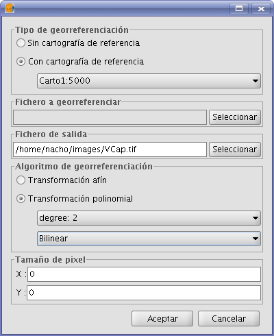
Start Dialogue georeferencing
To implement this type of georeferencing is imperative that we have previously charged in a view mapping that we will provide a geographic reference for taking control points. In case of not having it will close the options dialog georeferencing and proceed to prepare for the hearing. Once we have the view with reference maps georeferencing tool launched will see that the option "reference maps" is checked by default. Below is a dropdown menu which lists the views that gvSIG has at that time. If you have several it must select a view which is our base mapping for decision-points.
Dialog Georeferencing
In the panel marked "a georeferenced file" pops up a dialog for selecting the file for which you want to create checkpoints and later georeferencing.
The panel labeled "Output File" we must put the path and file name destination if the georeferencing is done with resampling. This option can vary from box options once we are inside the application, so it is not essential to a correct value at the moment, but if must be done before the end of the process.
The panel "georeferencing algorithm" select how we will get the output result. There are two possibilities, "affine transformation" and "polynomial transformation".
The affine transformation applied to raster an affine transformation only to the calculations performed with the control points taken. The affine transformation applied will be allocated "on the fly" for the display and the output image is the same as the input. The result of this transformation is therefore a georeferencing file. Keep in mind that this type of transformation is limited and the user will be responsible for selecting the most convenient transformation in each case.
The polynomial transformation involves a resampling of the input image taking into account the reference control points and obtaining an output image with deformations necessary to adapt to the new location. If you select this option we will be forced to decide the degree of transformation that we apply and the type of interpolation that we want to apply for calculating new pixels. Depending on whether you choose one degree or another need a minimum number of control points for them. This number of points required is given by the formula (order + 1) * (order + 2) / 2, ie for a polynomial of degree one will be needed at least three points, to grade two will need six points for third grade ten points ... The interpolation method affects the way we calculate the information that we have not. When an image georeferenced output image has deformations with respect to the original there are areas where no information is available. These can not be empty with what must be calculated from the areas where we know. These calculations can be performed by various methods, the simplest of these is "Nearest neighbor" which will be unknown pixel information closest known pixel. Other methods such as "bilinear" or "bicubic" make calculations using the known group of pixels surrounding the unknown. These other methods give a more relaxed but it is slower in its implementation. This option can vary from box options once we're inside the application.
The panel "Pixel Pitch" is the pixel size information of the output image. In principle this will be calculated from the input image but can be changed manually. This option can vary from box options once we are inside the application, so it is not essential to a correct value at this time.
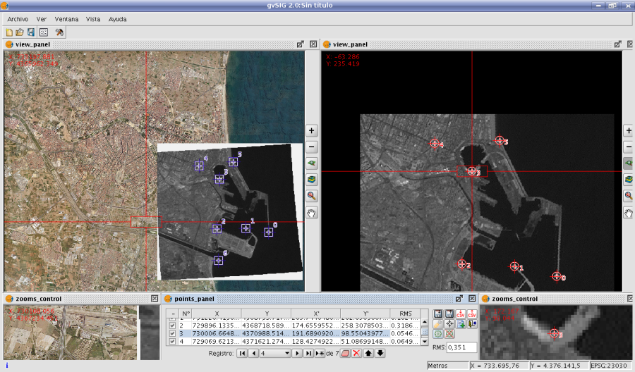
The views
Executing the application are two views. The left contains the base mapping that we carry in the gvSIG view of the right and the image we want to georeference. Both have a control bar on the right for view actions. Also in the upper left corner are the coordinates of the mouse cursor. In reference mapping coordinates are those of the real world. In the image to be georeferenced coordinates in pixel coordinate on the upper left.
Cursor Zoom
In the central part appears a cursor with a central window. The window cursor is active when the view can be resized and moved. The contents of this window will be on display in the zoom windows. Ca da vista has its associated zoom window at the bottom. Par resize window cursor select the view you want by clicking on it then bring the mouse to the edges of the window until the pointer changes to horizontal or vertical arrows. Now we click and drag to force the resizing. To move the cursor window select the view you want by clicking on it then bring the mouse to the corners of the window until the pointer changes by crossed arrows. We must now drag and drop to force displacement.
View Controls
There are six controls to handle the zoom level and position of the view mapping Increase the level of zoom: the zoom level increases by multiplying by 2 the current level.

Decrease zoom level: it decreases the zoom level by dividing by 2 the current level.

Zoom area selection: Activates a tool on the hearing in order to make a rectangle the area we want to see enlarged.

Full Zoom: Put a zoom level so that you can view the entire mapping.

Zoom Previous: Sets the zoom level that you previously selected.

Displacement: clicking and dragging on the scroll view mapping.

Zoom controls
Each view has an associated georeferencing zoom window centered over the cursor. When we move the cursor on the sale of view varies the position where the zoom and focus when we change the window size changes the zoom level. In the upper left corner of the window coordinates of the mouse cursor as in the overview.
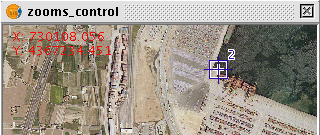
Zoom box associated with the views
Checkpoints
A control point is an entity that provides a correspondence between a geographic coordinate and pixel coordinate. Control points are represented in raster geographic view as Blue-and red circles respectively. To add a new control point is selecting "New" in the table control. This makes a new entry in the table appears. A control point is associated with a table entry. By selecting "New" automatically creates a point at coordinates 0, 0 for both views and will activate the tool "move point". Now clicking on the view point where we will move puncture. We assign the coordinate point numerically by writing directly on the input value in the table (X for the geographic coordinates X, Y geographic coordinate for Y, X 'for X and Y pixel coordinate' for the pixel Y coordinate). The points can also be moved by clicking and dragging on them. This may be done both in hearings and in the zooms.
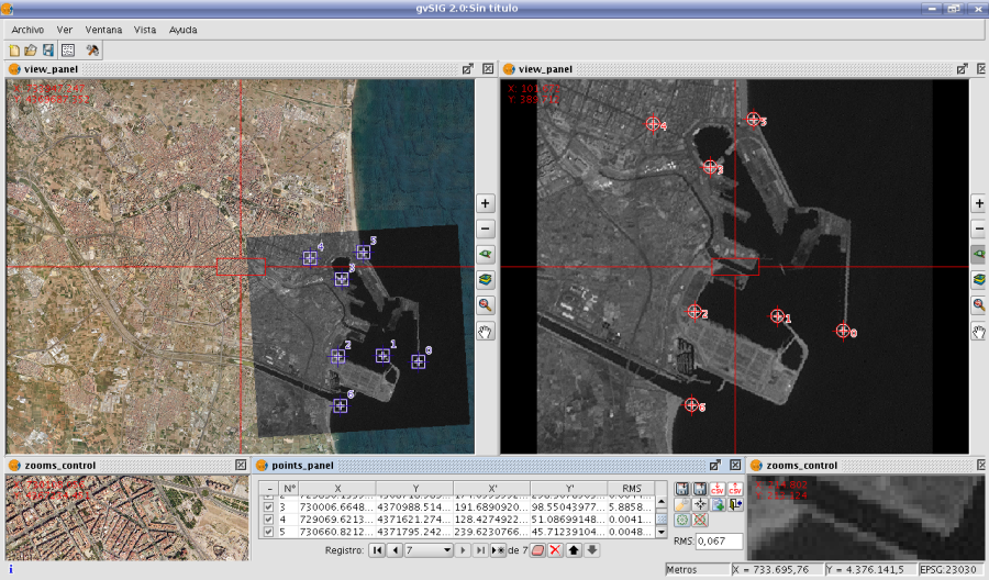
The process of georeferencing. Sights and points of control
Options
The panel labeled "Output File" we must put the path and file name destination if the georeferencing is done with resampling.
The panel georeferencing algorithm "select how we will get the output result. There are two possibilities, "affine transformation" and "polynomial transformation".
The affine transformation applied to raster an affine transformation only to the calculations performed with the control points taken. The affine transformation applied will be allocated on the fly for the display and the output image is the same as the input. The result of this transformation is therefore a georeferencing file. Keep in mind that this type of transformation is limited and the user will be responsible for selecting the most convenient transformation in each case.
The polynomial transformation involves a resampling of the input image taking into account the reference control points and obtaining an output image with deformations necessary to adapt to the new location. If you select this option we will be forced to decide the degree of transformation that we apply and the type of interpolation that we want to apply for calculating new pixels. Depending on whether you choose one degree or another need a minimum number of control points for them. This number of points required is given by the formula (order + 1) * (order + 2) / 2, ie for a polynomial of degree one will be needed at least three points, to grade two will need six points for third grade ten points ... The interpolation method affects the way we calculate the information that we have not. When an image georeferenced output image has deformations with respect to the original there are areas where no information is available. These can not be empty with what must be calculated from the areas where we know. These calculations can be performed by various methods, the simplest of these is "Nearest neighbor" which will be unknown pixel information closest known pixel. Other methods such as "bilinear" or "bicubic" make calculations using the known group of pixels surrounding the unknown. These other methods give a more relaxed but it is slower in its implementation.
The panel "Pixel Pitch" is the pixel size information of the output image. In principle this will be calculated from the input image but can be changed manually.
The panel labeled "Options" contains settings of a different nature. Since we can change the background color of view, the text color of the views. The "show the number of graphically checkpoint" will be displayed or hidden by the control point a point that indicates the corresponding point number. "Add the CSV file errors" will be generated when this type of text files with all the control points we can ignore the file or add the calculated errors. The "Focus the selected point view" makes automatically every time we select a point on the table the view is focused on this. The effect is much as if the tool center point was always active. The "error threshold for the warning," assigns the value at which the error appears in red on the table.
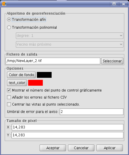
Options for georeferencing
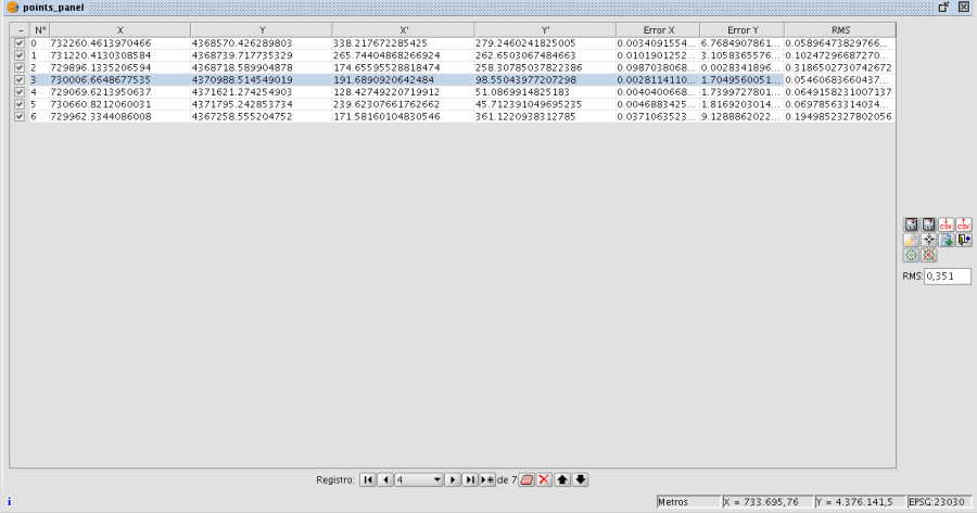
Points Table
The points table is below the sights and initially will be empty. Each table entry corresponds to a checkpoint. It appears all the information related to a point. This table can see it folded its default state or maximized. In its maximized state are folded more information. On the left side of the row there is a check to activate and deactivate the current row. This means that this point will not be displayed graphically or be taken into account for calculation errors and will be prosecuted to do a test. The information can be found in the points table on each point:
- Number of point
- Real coordinate X
- Real coordinate y
- Coordinate pixel X
- Coordinate pixel Y
- Error in X
- Error in Y
- Total RMS error for that point
The quality of the geometric correction can be estimated based on the mean square error RMS error and the contribution of each point. When the contribution to RMS of a point is high, this may indicate that the correspondence of points was poorly selected and the point is not well suited to model transformation between image and map or other information used as reference. The points with high contribution that exceeds a certain threshold can be deleted or deactivated, and calculate the RMS. However, when we are fully confident of the location of a point, and to find you, the RMS is triggered, it may be possible that the geometric model does not resolve the local arrangements, for which they may need a better model, which means, put some more points, right on the problem area.
There is also a global RMS error in an external text field for all points.
Control Panel points
Controls
Tool center point: When you press the focus control to the view point that is selected.

Georeferencing operation completes. Before you ask if we carry on the gvSIG view the results of the last trial. You'll also want confirmation of application output.

Launching the options dialog.

Make a test with the control points currently entered. If there are not enough for the specified algorithm will warn. The result is that applying the transformation and loading the transformed image on the view with the reference maps.

Save the control points in the metadata file attachment with the raster.

Retrieves the control points that are in the metadata file attached to raster.

Ends the test of processing the raster. Eliminate the test image loaded in the view with the mapping.

When the button "Select point" we are active, clicking on the view assigning the selected point on the table at that time to the position.

Sequence capture control points
There may be ways to capture control points with the tools available. An example would be the following sequence of actions:
- Click "New" in the table of control points. This will create a new row is selected in the table. In addition the tool "Move Point" is selected.
- Click with your mouse pointer over the view to locate the point raster.
- Click with your mouse pointer over the view with reference maps to locate the point.
- Push the button "Refocused selected view point" to place the checkpoint in the center and appears in the zoom window.
- With the tool of choice for area Zoom "or" increase the level of zoom "or" Decrease the zoom level "we can set the desired zoom level until the controls of" Zoom "we have an optimal resolution level approximate.
- Click and drag the control point in the zoom window to place it more precisely. The accuracy depend on how correct is selected previous zoom level.
- Use the zoom tools to return the view to a wider zoom level and to allow a new control point.
- To return to one point and reset the Selection Click on the row of the table, click "Center views the selected point, adjust the zoom level to zoom tools and we'll move the view by clicking and dragging on the window zoom for greater accuracy.
Georeferencing with resampling
Two types of processing for raster. If selected in the options the affine transformation the image obtained is not wide and applies an affine transformation on the view. This transformation is a scaling, displacement, rotation and deformation in the direction of axis X and / or Y axis The transformation with resampling involves generating a new image from the original on which areas can appear empty. These areas are due to the fact that the resulting image should be rectangular but the area covered by the data processing may not have applied this same way.
Results georeferenced image with resampling
Once the process of georeferencing the raster generated and loaded in the view we can apply a transparency per pixel to eliminate the empty areas.
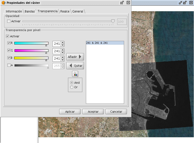
Image georeferenced, with application of transparency
Georeferencing without "Mapping Reference"
The georeferencing without reference maps is useful when you do not have imagery that guide us to assign the control points. We will have to allocate the actual coordinates directly by typing its value. In this case it is useful in view of the left so it will allow more space for the raster and the points table. The operation is very similar to the two views just that when you select the point on the reference maps have to type the entry of the table directly.
The operation of other controls is the same as with reference maps.


